First written April 2014.
Last modified March 2015.
Wikipedia has a great article about the Discrete Cosine Transform. These notes are laid out the way I learned about the topic, in the hope that someone will find it useful to see the same material presented in a different way.
Definition
The DCT-II is:
$$ X_k = \sqrt{2/N} s(k) \sum_{n=0}^{N-1} x_n cos \left[ \frac{\pi}{N} \left(n + .5\right)k \right] $$
Where:
- \(X\) is the DCT output.
- \(x\) is the input.
- \(k\) is the index of the output coefficient being calculated, from 0 to \(N-1\).
- \(N\) is the number of elements being transformed.
- \(s\) is a scaling function, \(s(y) = 1\) except \(s(0) = \sqrt{.5}\).
The DCT transforms input \(x\) to output \(X\). Both have the same number, \(N\), of elements.
A naïve implementation in C++:
void dct_ii(int N, const double x[], double X[]) {
  for (int k = 0; k < N; ++k) {
    double sum = 0.;
    double s = (k == 0) ? sqrt(.5) : 1.;
    for (int n = 0; n < N; ++n) {
      sum += s * x[n] * cos(M_PI * (n + .5) * k / N);
    }
    X[k] = sum * sqrt(2. / N);
  }
}
(dct_a.cc)
Variations
Sometimes you'll see the DCT without the \(\sqrt{2/N}\) or \(s(k)\) scale factors. The scaling makes the coefficients into an orthogonal matrix, which we'll cover later.
Sometimes \((n + .5) / N\) is spelled \((2n + 1) / 2N\). I've even seen a \(4N\) variant.
A gentle reminder that \(\sqrt{.5} = 1/\sqrt{2} = cos(\pi/4)\) because these terms keep popping up.
What does the DCT do?
The DCT transforms an input signal from the time domain into the frequency domain.
This compacts the energy of the signal, mostly into the low-frequency bins.
The DCT is used as a building block for many kinds of lossy compression for audio, video, and still images.
An over-simplified compressor:
- Take an input signal.
- Apply the DCT.
- Throw away some of the information. ("quantize" the DCT coefficients)
- Losslessly compress the coefficients.
- The compressed data should be smaller than losslessly compressing the original signal.
What is the DCT output?
The DCT transforms an input signal into a combination of cosine waves.
The first DCT coefficient (\(X_0\)) is sometimes called the "DC component" of the signal (DC as in direct current) because it's proportional to the average of all the input samples.
Each output coefficient corresponds to a DCT basis function. These functions are cosine waves of increasing frequencies.
If you multiply each basis function by its corresponding coefficient, their sum will be a reconstruction of the original input. This process is called the Inverse DCT and we'll cover it later.
The Discrete Fourier Transform (DFT) returns complex numbers. The DCT is equivalent to the real part of the DFT output.
The rest of this article deals specifically with an eight-point DCT-II, which is what JPEG compression is built on top of. Here is what the eight basis functions look like:
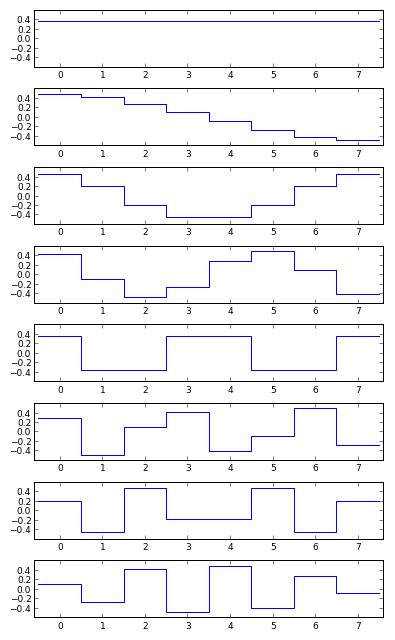
(source code: basis.py)
Matrix of coefficients
You can look at the DCT as a matrix multiplication where the inputs and outputs are row-vectors:
$$X = x \times M$$
For brevity, let's define:
$$ c_0 = \sqrt{.5} \times \sqrt{2/N}\\ c_j = cos\left(\pi j / 16\right) \times \sqrt{2/N} $$
The coefficient matrix is just the \(N \times N\) cosines and scale factors:
We don't need to calculate quite so many coefficients because e.g. \(c_{33} = c_1\).
After using circle symmetry to transform all the angles to the first quadrant, only eight unique coefficients are needed for an eight-point DCT:
Due to the scale factors, the coefficient matrix is an orthogonal matrix, meaning:
- All row vectors are unit vectors. ("normal" vectors)
- All row vectors are also orthogonal to each other. (i.e. the dot product of any two row vectors is zero)
- All column vectors are also orthonormal.
- The matrix can be inverted by transposing it. This is how we get to the Inverse DCT.
(Python script to measure this: ortho.py)
Implementation of an eight-point DCT
dct_b.cc is the same as the naïve implementation in dct_a.cc, but with the size hardcoded to eight. Compiled with g++ version 4.6.4 or 4.7.4 and flags -S -O3 -march=core-avx-i -masm=intel, the generated code looks like:
_Z8dct_ii_8PKdPd:
  vmovsd  xmm0, QWORD PTR [rdi+24]
  vmovsd  xmm4, QWORD PTR .LC1[rip]
  vaddsd  xmm0, xmm0, QWORD PTR [rdi+8]
  vmovsd  xmm2, QWORD PTR .LC2[rip]
  vmovsd  xmm8, QWORD PTR .LC3[rip]
  vaddsd  xmm0, xmm0, QWORD PTR [rdi+32]
  ; and on and on...
  ; eventually some "vmulsd" instructions, but no "call"s
The optimizer has fully unrolled the two nested loops, and evaluated all the calls to cos() and sqrt(). There are no branches, just a linear run of AVX instructions. Counting:
$ awk '{print $1}' < dct_b.s | grep 'v....d' | sort | uniq -c
     64 vaddsd
     53 vmovsd
     72 vmulsd
      1 vxorpd
With -ffast-math:
     56 vaddsd
     54 vmovsd
     64 vmulsd
(An aside: g++ versions 4.8.3 and 4.9.1 produce different output with calls to cos. The rest of this article uses 4.7)
The optimizer generates 46 constants, but only eight unique constants are needed in the matrix approach. Some of this is due to floating point inaccuracy: c1 and c31 should evaluate to the same number but their mantissas are different by one ulp. This is illustrated by constants.cc.
Generating better code
I can make the compiler generate better code by writing out the matrix multiplication in full:
static const double c0 = 1. / sqrt(2.) * sqrt(2. / 8.);
static const double c1 = cos(M_PI * 1. / 16.) * sqrt(2. / 8.);
static const double c2 = cos(M_PI * 2. / 16.) * sqrt(2. / 8.);
static const double c3 = cos(M_PI * 3. / 16.) * sqrt(2. / 8.);
static const double c4 = cos(M_PI * 4. / 16.) * sqrt(2. / 8.);
static const double c5 = cos(M_PI * 5. / 16.) * sqrt(2. / 8.);
static const double c6 = cos(M_PI * 6. / 16.) * sqrt(2. / 8.);
static const double c7 = cos(M_PI * 7. / 16.) * sqrt(2. / 8.);

#define a x[0]
// etc

void dct_ii_8a(const double x[8], double X[8]) {
  X[0] = a*c0 + b*c0 + c*c0 + d*c0 + e*c0 + f*c0 + g*c0 + h*c0;
  X[1] = a*c1 + b*c3 + c*c5 + d*c7 - e*c7 - f*c5 - g*c3 - h*c1;
  X[2] = a*c2 + b*c6 - c*c6 - d*c2 - e*c2 - f*c6 + g*c6 + h*c2;
  X[3] = a*c3 - b*c7 - c*c1 - d*c5 + e*c5 + f*c1 + g*c7 - h*c3;
  X[4] = a*c4 - b*c4 - c*c4 + d*c4 + e*c4 - f*c4 - g*c4 + h*c4;
  X[5] = a*c5 - b*c1 + c*c7 + d*c3 - e*c3 - f*c7 + g*c1 - h*c5;
  X[6] = a*c6 - b*c2 + c*c2 - d*c6 - e*c6 + f*c2 - g*c2 + h*c6;
  X[7] = a*c7 - b*c5 + c*c3 - d*c1 + e*c1 - f*c3 + g*c5 - h*c7;
}
Without -ffast-math, this generates the expected 64 multiplications. This number can be brought down by manually factoring, e.g.:
-  X[0] = a*k0 + b*k0 + c*k0 + d*k0 + e*k0 + f*k0 + g*k0 + h*k0;
+  X[0] = (a + b + c + d + e + f + g + h)*k0;
Further multiplications can be traded for additions by exploiting "rotation"-like operations:
$$ \begin{eqnarray} y_0 & = & a x_0 + b x_1 & = & (b - a) x_1 + a (x_0 + x_1)\\ y_1 & = - & b x_0 + a x_1 & = - & (a + b) x_0 + a (x_0 + x_1) \end{eqnarray} $$
For example:
-  X[2] = adeh*c2 + bcfg*c6;
-  X[6] = adeh*c6 - bcfg*c2;
+  const double adeh26 = adeh * (c2 + c6);
+  X[2] = (bcfg - adeh)*c6 + adeh26;
+  X[6] = adeh26 - (bcfg + adeh)*c2;
There are three variants of the DCT code in dct_c.cc. The last one generates:
     20 vaddsd
     22 vmovsd
     17 vmulsd
     18 vsubsd
I think that's as far as naïve algebraic factoring will go. A smarter approach is needed to further reduce the work. The LLM algorithm (described later) claims it can get this down to 11 multiplies and 29 adds.
But first:
Inverse DCT
The inverse of the DCT-II is the DCT-III. Its coefficient matrix is the transpose (rows become columns) of the DCT-II matrix. Or, if you prefer, the forward and inverse transforms are:
$$ X_k = \sqrt{2/N} s(k) \sum_{n=0}^{N-1} x_n cos \left[ \frac{\pi}{N} \left(n + .5\right)k \right]\\ x_n = \sqrt{2/N} \sum_{k=0}^{N-1} s(k) X_k cos \left[ \frac{\pi}{N} \left(n + .5\right)k \right]\\ $$
A naïve implementation in C++:
void idct(int N, const double X[], double x[]) {
  for (int n = 0; n < N; ++n) {
    double sum = 0.;
    for (int k = 0; k < N; ++k) {
      double s = (k == 0) ? sqrt(.5) : 1.;
      sum += s * X[k] * cos(M_PI * (n + .5) * k / N);
    }
    x[n] = sum * sqrt(2. / N);
  }
}
(dct_a.cc)
The LLM DCT
There's a faster DCT algorithm, sometimes called LLM for its authors: Loeffler, Ligtenberg, and Moschytz.
It's described in their 1989 paper "Practical Fast 1-D DCT Algorithms with 11 Multiplications" (see the "Further reading" section below) but here's the relevant part:
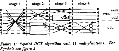
There's an important mistake above: \(\sqrt2c1\) should read \(\sqrt2c6\) or you will not be computing a DCT.
Here's how to interpret the block diagram:
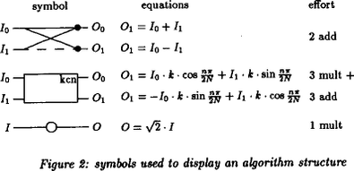
(nit: they write \(O_1\) twice, obviously the first instance should read \(O_0\))
They count rotations as "3 mult + 3 add" because they're using an optimization that works for fixed angles. You can read more about it in my rotation notes.
Here's my implementation of the LLM DCT: llm_dct.cc
In the LLM paper, the authors choose to scale the DCT by \(\sqrt{2}\) instead of \(\sqrt{2/N}\), so the result of their DCT isn't normalized. This is okay if you do the scaling as part of a later quantization step, or if you build an IDCT that expects the different scaling. In my implementation, I've added the eight divides by \(\sqrt{N}\) to get normalized output that I can compare to the naïve implementation.
My implementation, compiled without -ffast-math:
     19 vaddsd  ; plus 10 subs makes 29, as claimed.
      8 vdivsd  ; this is due to scaling I added.
     18 vmovsd
     11 vmulsd  ; as claimed.
     10 vsubsd
My code looks like Single Static Assignment form whereas other implementations (like llm_mit.cc) tend to define nine variables and juggle the computation between them.
In my opinion, the juggling makes the signal path harder to follow. In my testing, both implementations result in the same number of assembler instructions emitted.
The AAN DCT
Another fast DCT algorithm is AAN, named for its authors: Arai, Agui and Nakajima. Their paper, "A fast DCT-SQ scheme for images" gets cited often but I can't find it online and I think it might be written in Japanese. Their algorithm uses five multiplies (plus eight post-multiplies for scaling, which they argue don't count because they can be moved into the quantization matrix).
Here's a diagram of the AAN DCT taken from page 52 of the JPEG: Still Image Data Compression Standard text book my William B. Pennebaker and Joan L. Mitchell:
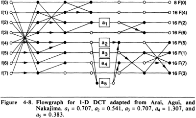
This is my implementation: aan.cc
Compiled with -ffast-math:
     15 vaddsd ; plus 14 subs makes 29.
     18 vmovsd
     13 vmulsd ; 5 from AAN, plus 8 from scaling I added.
     14 vsubsd
The book gives numeric constants, which are are easy to replace with symbolic ones when you know what to look for: cosines and square roots.
The post-scaling factors can be determined numerically by dividing DCT output by AAN output, or algebraically by following the code.
Further reading
There are many papers about implementing fast DCTs. Many of them are written by awesome electrical engineers who draw block diagrams and measure the depth of the signal path and then go implement it all in silicon.
Practical Fast 1-D DCT Algorithms with 11 Multiplications is the LLM paper: it reviews several previous algorithms and gives a newer and more compact one. It was published in 1989.
A Fast Computational Algorithm for the Discrete Cosine Transform is from 1977, and has an awesome block diagram of 4-point through 32-point DCTs on the last page.